A Brief intro to Gaussian Processes

• Gaussian Processes are a fascinating tool for usage in RL due to modelling uncertainty and data efficiency
• I briefly introduced GP’s and shown how/why they are used in RL

Gaussian processes (GPs) are a fascinating tool in the machine learning toolbelt. They stand out for a couple of reasons: some people will like them for their data efficiency, others love them for their ability to incorporate domain knowledge and yet others will love them for their visual or mathematical beauty. I was first introduced with GPs when studying ways to optimize chatbots or dialogue agents using data. In this blog post, I will introduce some of the concepts of GPs, discuss their strengths and weaknesses and discuss some applications in Reinforcement Learning (RL).

Before diving in to the details of the GP model, it’s important to understand that GPs are a form of Bayesian machine learning. This means that they allow for some sort of upfront knowledge to be encoded into a prior. Another thing to consider is that GPs are non-parametric: the number of parameters of the model is not fixed but depends on the size of the training set, similarly to e.g. the k-nearest neighbours and support vector machine models. A final thing to note about GPs is that they provide a full probability distribution instead of single predictions such as provide by maximum likelihood estimation (mle) or its Bayesian friend maximum a posteriori estimation (map).

The Gaussian Process

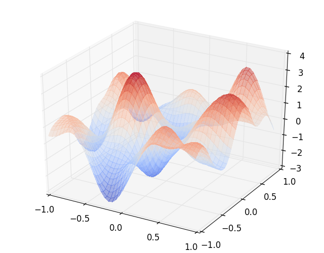
Hoping not to have scared anyone off with all of this jargon, let’s retry with some definitions: “A Gaussian Process is a collection of random variables, any finite number of which have a joint Gaussian distribution.”¹ Formally, some function \(f(x)\) over a set \(X\) follows a GP distribution as defined by some mean \(\mu\) and a covariance function or kernel \(k(x, x’)\): $$f(x) \sim \mathcal{GP}(\mu(x), k(x, x’)), \forall xx’ \in X \\\ \mu(x) = \mathbb{E}[f(x)] \\\ k(x, x’) = \mathbb{E}[(f(x) - \mu(x))(f(x’) - \mu(x’))] $$ A simple example of a GP is visualized in Figure 2. Here, \(X = \mathbb{R}\) and \(f(x) = Y \).

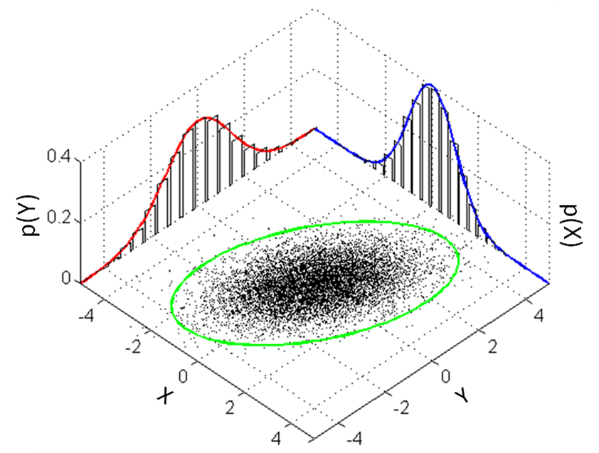
Having checked the definition and a simple example of a GP, we now turn to some of the things you can (mathematically) do with GPs. We focus on the manipulations that are useful when doing predictions. For starters, we have already seen that we can extract single-variable \(\mu\)s from the joint distribution. We can do the same for the covariance matrix (kernel) and obtain the individual distributions: $$ \mu = \begin{bmatrix} \mu_{X} \\ \mu_{Y} \end{bmatrix}, \Sigma = \begin{bmatrix} \Sigma_{XX} & \Sigma_{XY} \\ \Sigma_{YX} & \Sigma_{YY} \end{bmatrix} $$ Extracting distributions for \(X\) and \(Y\): $$ X \sim \mathcal{N}(\mu_{X}, \Sigma_{XX}) \\ Y \sim \mathcal{N}(\mu_{Y}, \Sigma_{YY}) $$ This manipulation is commonly known as marginalization.

Another manipulation that is useful for prediction is conditioning. Conditioning boils down to expressing the distribution of one variable in terms of the distribution of the other. The full derivation is too much for this blog post², but this is the information you’ll need in order to do so: $$ \begin{align} Y | X \sim \mathcal{N}( & \mu_{Y} + \Sigma_{YX} \Sigma_{XX}^{-1}(X - \mu_X), \\\ & \Sigma_{YY} - \Sigma_{YX} - \Sigma_{YX}\Sigma_{XX}^{-1}\Sigma_{XY}) \end{align} $$ In supervised prediction settings with target variable \(Y\), \(\Sigma\) and \(\mu_Y\) can be estimated based on the training set and predictions on input \(X\) can be made.³ Note that \(Y\) is a full distribution rather than a mle or map. So far, we have seen that a GP is a distribution over functions with mean \(\mu\) and kernel \(k(x, x’)\) and can be understood as a generalization of a multivariate Gaussian distribution. How can we actually fit it to a data set and use for predictions though?

GP Regression

Let’s consider using GPs for regression. The task in regression is to estimate some target function \(f(X) \to y, y \in \mathbb{R}\) using a set of pairs \(X’, y’\) (the training set) and then use the estimated \(\hat{f}\) to predict the values \(y^*\) for a test set \(X^*\). In most regression tasks, \(y’\) is measured using some imprecise sensors and comes with a measurement error. This error can be expressed using an assumed independent error term \(\epsilon\) with variance \(\sigma\). The full model then becomes: $$ \begin{align} f(x) & \sim \mathcal{GP}(\mu, K), x \in X \\\ \epsilon & \sim \mathcal{N}(0, \sigma_n^2I) \text{ indep. of }f(x) \\\ y_i & = f(x_i) + \epsilon_i \\\ \overbrace{x_1, \dots, x_\ell}^{\text{unobserved}: (X,y)^*} & , \overbrace{x_{\ell+1}, \dots, x_n}^{\text{observed:}(X,y)’} \in S \\\ y_1, \dots, y_\ell ~&,~ y_{\ell+1}, \dots, y_n \in \mathbb{R} \\\ \mu_{x_1}, \dots ~&,~ \dots, \mu_{x_n} \end{align} $$

The next step in the regression process consists of applying the marginalization and conditioning operations in a meaningful way. Marginalization gives: $$ \begin{bmatrix} y’ \\ y^* \end{bmatrix} \sim \mathcal{N}(\mu, \begin{bmatrix} K(X’,X’)+\sigma^2_nI & K(X’, X^*) \\ K(X^*, X’) & K(X^*, X^*) \end{bmatrix}) $$ Conditioning on the training set \(X’, y’\) and the known test points \(X^*\) gives: \begin{align} y^*|X’, y’, X^* \sim &~ \mathcal{N}(\hat{\mu}, K(X^*, X^*) - K(X^*, X’)[K(X’, X’) + \sigma^2_nI]^{-1}K(X’, X^*) \\\ \end{align} Typically, the input can be transformed so that \(\mu = 0\), in which case $$ \hat{\mu} = \mathbb{E}[y^*|X’, y’, X^*] = K(X^*, X’)[K(X’, X’) + \sigma^2_nI]^{-1}y' $$ Neat, we now have an expression of the full distribution over values to be predicted \(y^*\)! This is something not many ml models offer out of the box. We can obtain a point-estimates with confidence intervals by looking at the expecation and standard deviation at a particular \(y^*_i\). All we need now is to get our hands on a training set \(X’, y’\) and some evaluation set of interest \(X^*\) and make some estimate for the error term \(\sigma^2_n\). Oh, and we need to define which kernel \(K\) fits our domain well.

Domain knowledge and kernels

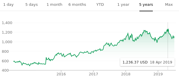
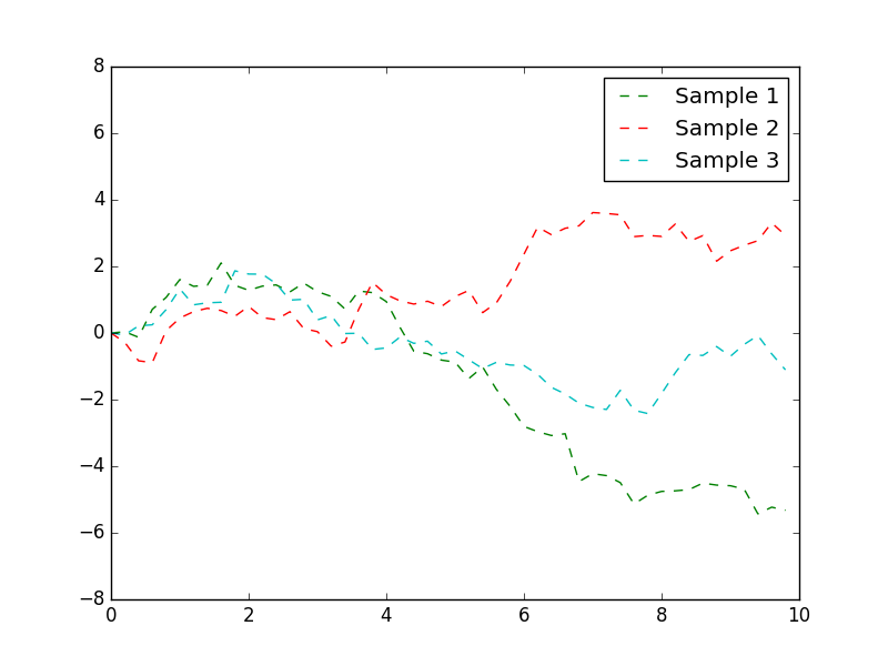
I already mentioned that GPs are a Bayesian method and allow for integrating domain knowledge into the model through a prior. Where can we put upfront knowledge in GPs? We might know something about the \(\mu\), should we encode something on this into the model? This sounds like a good idea, but in practice it is much easier to normalize the entire dataset so that each \(\mu = 0\). What about a prior on the kernel? Let’s have a look at an example in which we would like to predict stock prices. Let’s think about what we know about stock markets, let’s consider what a stock market stock size could look like in Figure 3.

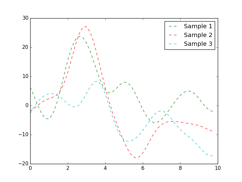
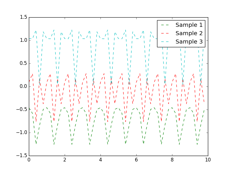
It is quite clear that the random walk kernel in Figure 4(b). So when doing an estimation of the stock price in the future, or in between sampled times, it would be a great idea to encode domain knowledge using that kernel.

Gaussian Processes and Reinforcement Learning

Regression based on Gaussian processes can be used quite effectively within various Reinforcement Learning approaches. For example, when estimating transitions in model-based RL[^4].

Gaussian processes can also used to estimate (V) and (Q) functions within e.g. dialogue management and for personalization with RL.